Chapter 3 Data Introduction
Data preprocessing is one of the most important steps for our research. The quality of data preprocessing is directly related with quality of the data analysis. Most of time, the raw data is really messy and disorganized. What I need to is to make the data organized and split it into different data tables for different analysis. For one data table, life is easy because all I need to do is to put variable of interest into a huge matrix. For multiple data table, I need to split it into different data tables based on their basic features (variables measuring similar features, such as friends number and social network size). Most importantly, I need to make a design matrix for the data table, aka grouping strategy. Based on different grouping strategies, we can have completely different results in our plot and conclusion. However, it is totally up to you to choose the grouping variables: in my current data set, I can group participants according to their social intelligence, general intelligence, age, sex, gpa, and so on. It is highly recommended to read related article before choose the best group variables for your analysis.
In the rest of this chapter, I will introduce three data sets used in this book, Collective Action Data set, Low Income Sausage and Wines. The main data set is corresponding to PCA, BADA, PLS, MCA, MFA; The second one is for CA and the last one is for DiSTATIS.
3.1 Main data set: Collective Action Data Set
The main data set we are using is from an research article published on PNAS last year. Several part of different data tables consist the data set:
- The first part is experimental data:
- The game performance for each round
- The time usage for each round
- Emotional & Social Intelligence test
- State of reasoning
- Comprehension
- Spontaneous
- Academic results
- SAT&ACT overall
- SAT&ACT Math
- SAT&ACT Verbal
- GPA
- Attitude
- Global_warming
- Government
- Environmental ecology
- Social relationship
- Close friends number
- Social network size
- Personality
- Helpful
- Trust
- Hard working
- Volunteer
- Take advantage
- Demographoc
- Age
- Sex
- Parent Education
- Parents’ job1
- Parents’ job2
- Race
- Income
- Language
- Major
- religious
- Emotional processing ability
- Eyetest scores
- Quizzes scores
All these variables are easy to understand except the experiment and emotional processing abilities. Generally, the experiment is a token collection game. Its aim is to collect token as many as possible. The token will automatically generate following a rule. If you and your teammates are following this rule to play the game, you will have higher generate rate of the token during this game; However, if you don’t follow it, you will end the game soon with less number of tokens in your packet.
For the emotional processing ability, it used a classic paradigm in psychology: participants are required to watch only eyes parts of many face pictures and make decision on what’s the emotions on the faces behind. For the social intelligence part, it is similar but participants are required to read paragraphs and make response, which is called Short Story Test (SST), to measure how much capacity participants can empathize with others.
All these variables have detailed illustration on website. Please see this supplementary information document in PNAS. In my data preprocessing, you will notice that I only use Negative Condition as example in this book. The reason why I didn’t include Positive and Negative two conditions is that I am running out of time to submit my final project… Definitely I will finish it after the class.
- Negative Condition: R1-R3, HIGH resource, LOW group members; R4-R6, LOW resource, HIGH group members
- Positive Condition: R1-R3, LOW resource, HIGH group members; R4-R6, HIGH resource, LOW group members
In the following chunk, I showed a detailed process of how I did data cleaning and preprocessing in raw data (raw data can be downloaded here 1.3).
# Data preprocessing----
load(url("https://github.com/yilewang/MSA/blob/main/Dataset/CogCollect.RData?raw=true"))

# Data Cleaning: Missing values
rownames(data.tab3) <- 1:360
data.tab3$q2[212] <- 3.08
data.tab3$q2[300] <- 1.7

# Binding all the data sets
all.cog <- cbind(data.frame(data.info_demo), data.frame(data.pca), data.frame(data.tab2[3:8]),
 data.frame(data.tab3[3:19]))

all.cog <- all.cog[order(all.cog[, "ANumber"]), ]
rownames(all.cog) <- c(1:360)

# Give Colnames
colnames(all.cog)[46:59] <- c("age", "GPA", "close_friends", "social_network", "instruction",
 "take_advantage", "helpful", "trust", "volunteer", "global_warming", "hard_work",
 "government", "environment_eco", "parent_edu")

colnames(all.cog)[18:25] <- c("religions", "language", "races", "incomes", "majors",
 "sex", "parent_job_1", "parent_job_2")

# create sub data tables
sub.token.collection <- cbind(all.cog[, 26:27], all.cog[, 30:36])

sub.token.collection.time <- cbind(all.cog[, 26:27], all.cog[, 37:42])

sub.empathy <- cbind(all.cog[, 26:27], all.cog[, 43:45], all.cog[, "Spontaneous"])
colnames(sub.empathy)[6] <- "Spontaneous"


sub.emotion <- cbind(all.cog[, 26:27], all.cog[, 28:29])

sub.personality <- cbind(all.cog[, 26:27], all.cog[, 51:54], all.cog[, 56])
colnames(sub.personality)[7] <- "hard_work"

sub.attitude <- cbind(all.cog[, 26:27], all.cog[, 55], all.cog[, 57:58])
colnames(sub.attitude)[3] <- "global_warming"

sub.friends <- cbind(all.cog[, 26:27], all.cog[, 48:49])

sub.demographic <- cbind(all.cog[, 26:27], all.cog[, 46], all.cog[, 18:25], all.cog[,
 "parent_edu"])
colnames(sub.demographic)[12] <- "parent_edu"
colnames(sub.demographic)[3] <- "age"


## ****ACT converts to SAT**** ACT DATA
ACT.math.table <- all.cog[which(all.cog$ACT.MATH.SCORE < 40), ]
ACT.reading.table <- all.cog[which(all.cog$ACT.READING.SCORE < 40), ]
ACT.english.table <- all.cog[which(all.cog$ACT.ENGLISH.SCORE < 40), ]
# ACT_MATH
ACT.math <- cbind(as.matrix(ACT.math.table$ANumber), as.matrix(ACT.math.table$ACT.MATH.SCORE))
# ACT_Verbal
ACT.verbal <- matrix(0, nrow = length(ACT.english.table$ACT.ENGLISH.SCORE))
for (i in 1:length(ACT.english.table$ACT.ENGLISH.SCORE))
{
 ACT.verbal[i] <- sum(ACT.reading.table$ACT.READING.SCORE[i] + ACT.english.table$ACT.ENGLISH.SCORE[i])
}
ACT.verbal <- cbind(as.matrix(ACT.reading.table$ANumber), ACT.verbal)
# SAT DATA
SAT.math.table <- all.cog[which(all.cog$SAT.MATH.SCORE < 801), ]
SAT.verbal.table <- all.cog[which(all.cog$SAT.VERBAL.SCORE < 801), ]
# SAT_MATH
SAT.math <- cbind(as.matrix(SAT.math.table$ANumber), as.matrix(SAT.math.table$SAT.MATH.SCORE))
# SAT_VERBAL
SAT.verbal <- cbind(as.matrix(SAT.verbal.table$ANumber), as.matrix(SAT.verbal.table$SAT.VERBAL.SCORE))
# Create a calculator to convert ACT to SAT Read data from github
x.math <- getURL("https://raw.githubusercontent.com/yilewang/MSA/main/Dataset/ACT_MATH.csv")
math_con <- read.csv(text = x.math)
colnames(math_con)[1] <- "ACT_MATH"  ## Avoid UTF-8 error
x.verbal <- getURL("https://raw.githubusercontent.com/yilewang/MSA/main/Dataset/ACT_VERBAL.csv")
verbal_con <- read.csv(text = x.verbal)
colnames(verbal_con)[1] <- "ACT_VERBAL"  ## Avoid UTF-8 error
# Create a workspace to store the new MATH and VERBAL info
act.math.con <- ACT.math
act.verbal.con <- ACT.verbal
act.comp.con <- cbind(all.cog[, 26], all.cog[, 7])
colnames(act.comp.con) <- c("ANumber", "Composite")
# Make a calculator to convert ACT scores to SAT scores
calculator.math <- function(score)
{
 index <- which(math_con == score)
 return(math_con[index, 2])
}
calculator.verbal <- function(score)
{
 index <- which(verbal_con == score)
 return(verbal_con[index, 2])
}
# For loop to convert the ACT score to SAT score
for (i in 1:length(ACT.math[, 1]))
{
 act.math.con[i, 2] <- calculator.math(ACT.math[i, 2])
}

for (i in 1:length(ACT.verbal[, 1]))
{
 act.verbal.con[i, 2] <- calculator.verbal(ACT.verbal[i, 2])
}
for (i in 1:length(all.cog[, 1]))
{
 act.comp.con[i, 2] <- calculator.math(all.cog$ACT.COMPOSITE.SCORE[i])
}


# Merge data
MATH <- rbind(act.math.con, SAT.math)
VERBAL <- rbind(act.verbal.con, SAT.verbal)
COMP <- act.comp.con
# Get the RANK
MATH <- MATH[order(MATH[, 1]), ]
MATH <- MATH[-54, ]
VERBAL <- VERBAL[order(VERBAL[, 1]), ]
VERBAL <- VERBAL[-54, ]
COMP <- COMP[order(COMP[, 1]), ]
sub.grades <- cbind(all.cog[, 26:27], COMP[, 2], MATH[, 2], VERBAL[, 2], all.cog$GPA)
colnames(sub.grades)[6] <- "GPA"
colnames(sub.grades)[3:5] <- c("SAT.COMP", "SAT.MATH", "SAT.VERBAL")


# the data we can use for our analysis
data.to.use <- cbind(sub.token.collection[, 1:8], sub.token.collection.time[, 3:8],
 sub.friends[, 3:4], sub.grades[, 3:5], sub.empathy[, 3:6], sub.personality[,
  3:7], sub.attitude[, 3:5])
supplement.token <- cbind(all.cog[, 26], all.cog[, 36])
colnames(supplement.token)[1:2] <- c("ANumber", "total_earning")
supplement.token <- as.data.frame(supplement.token)

sub.group <- matrix(0, ncol = 4, nrow = 360)
colnames(sub.group) <- c("gpa", "emo", "group", "col")
rownames(sub.group) <- 1:360
sub.group <- cbind(all.cog[, 26:27], sub.group)

# Grouping variable: GPA
sub.gpa <- cbind(all.cog[, 26:27], all.cog$GPA)
colnames(sub.gpa)[3] <- "general"
quan.gpa <- quantile(as.numeric(all.cog$GPA), seq(0, 1, 1/3))
under <- which(sub.gpa[, 3] <= quan.gpa[2])
between <- which(sub.gpa[, 3] > quan.gpa[2] & sub.gpa[, 3] <= quan.gpa[3])
over <- which(sub.gpa[, 3] > quan.gpa[3])
sub.group[, 3][under] <- 1
sub.group[, 3][between] <- 2
sub.group[, 3][over] <- 3


# Grouping variable: Emo
sub.emo <- cbind(all.cog[, 26:27], all.cog$EyesTestScore)
colnames(sub.emo)[3] <- "general"
quan.emo <- quantile(as.numeric(all.cog$EyesTestScore), seq(0, 1, 1/3))
under <- which(sub.emo[, 3] <= quan.emo[2])
between <- which(sub.emo[, 3] > quan.emo[2] & sub.emo[, 3] <= quan.emo[3])
over <- which(sub.emo[, 3] > quan.emo[3])
sub.group[, 4][under] <- 100
sub.group[, 4][between] <- 200
sub.group[, 4][over] <- 300

# spearman correlation results > 0.90
spearman.gpa <- cor(sub.gpa[, 3], sub.group[, 3], method = "spearman")
spearman.emo <- cor(sub.emo[, 3], sub.group[, 4], method = "spearman")

print(paste("corr gpa:", spearman.gpa))
[1] "corr gpa: 0.931355248926045"[1] "corr emotional 0.945673602462476"sub.group[, 5] <- sub.group[, 3] + sub.group[, 4]
# for each condition low-median-high
condition1 <- which(sub.group[, 5] == 101)
condition2 <- which(sub.group[, 5] == 102)
condition3 <- which(sub.group[, 5] == 103)
condition4 <- which(sub.group[, 5] == 201)
condition5 <- which(sub.group[, 5] == 202)
condition6 <- which(sub.group[, 5] == 203)
condition7 <- which(sub.group[, 5] == 301)
condition8 <- which(sub.group[, 5] == 302)
condition9 <- which(sub.group[, 5] == 303)
# give names
sub.group[, 5][condition1] <- "LS_LG"
sub.group[, 5][condition2] <- "LS_MG"
sub.group[, 5][condition3] <- "LS_HG"
sub.group[, 5][condition4] <- "MS_LG"
sub.group[, 5][condition5] <- "MS_MG"
sub.group[, 5][condition6] <- "MS_HG"
sub.group[, 5][condition7] <- "HS_LG"
sub.group[, 5][condition8] <- "HS_MG"
sub.group[, 5][condition9] <- "HS_HG"
# choose 4 conditions
sub.conditions.1 <- sub.group[which(sub.group[, 5] == "LS_LG"), ]
sub.conditions.2 <- sub.group[which(sub.group[, 5] == "HS_LG"), ]
sub.conditions.3 <- sub.group[which(sub.group[, 5] == "HS_HG"), ]
sub.conditions.4 <- sub.group[which(sub.group[, 5] == "LS_HG"), ]
# put them into a group
sub.conditions.1$group <- as.factor(sub.conditions.1$group)
sub.conditions.2$group <- as.factor(sub.conditions.2$group)
sub.conditions.3$group <- as.factor(sub.conditions.3$group)
sub.conditions.4$group <- as.factor(sub.conditions.4$group)
# make sub condition and organize them
sub.condition <- rbind(sub.conditions.1, sub.conditions.2, sub.conditions.3, sub.conditions.4)
data.to.use.sup <- cbind(data.to.use, supplement.token$total_earning)
colnames(data.to.use.sup)[32] <- "total_earning"
final.table <- merge(sub.condition, data.to.use.sup, by = "ANumber")
final.table <- select(final.table, -c("SessionType.y"))
names(final.table)[names(final.table) == "SessionType.x"] <- "SessionType"
### ________________________________________### different conditions, the two
### condition, postive and negative we can use for analysis
exp.neg <- final.table[which(final.table$SessionType == "Low_High" | final.table$SessionType ==
"8.4"), ]
exp.pos <- final.table[which(final.table$SessionType == "High_Low" | final.table$SessionType ==
"4.8"), ]
## color
index <- prettyGraphsColorSelection(n.colors = 4, starting.color = sample((1:300),
4))
# manually setting color design
m.color.design <- as.matrix(colnames(exp.neg[8:36]))
m.color.design[1:3] <- prettyGraphsColorSelection(starting.color = sample(1:170,
1))
m.color.design[4:6] <- prettyGraphsColorSelection(starting.color = sample(1:170,
1))
m.color.design[7:9] <- m.color.design[1:3]
m.color.design[10:12] <- m.color.design[4:6]
m.color.design[13:14] <- prettyGraphsColorSelection(starting.color = sample(1:170,
1))
m.color.design[15:17] <- prettyGraphsColorSelection(starting.color = sample(1:170,
1))
m.color.design[18:21] <- prettyGraphsColorSelection(starting.color = sample(1:170,
1))
m.color.design[22:26] <- prettyGraphsColorSelection(starting.color = sample(1:170,
1))
m.color.design[27:29] <- prettyGraphsColorSelection(starting.color = sample(1:170,
1))
### ________________________________________###
## **** ending of the data preprocessing ****It is worth to mention that the chunk above is the data preprocessing for quantitative data.
We used similar strategy for qualitative data preprocessing. The essential part of qualitative data coding is that I need to convert all the quantitative data into categorical format (1,2,3) by using quantile function. I already compile a new function for the bin coding, please see Function Chapter2.8 in this book.
bins.exp.neg <- as.data.frame(exp.neg)
for(i in 7:26){
  bins.exp.neg[,i] <- bins_helper(bins.exp.neg[,i],
                                  colnames(bins.exp.neg)[i])
}
## R1 spearman r: 0.9425675
## R2 spearman r: 0.9433265
## R3 spearman r: 0.9408037
## R4 spearman r: 0.9436019
## R5 spearman r: 0.9418503
## R6 spearman r: 0.9436669
## R1.TimeLeft spearman r: 0.9446858
## R2.TimeLeft spearman r: 0.9502324
## R3.TimeLeft spearman r: 0.9486652
## R4.TimeLeft spearman r: 0.9481581
## R5.TimeLeft spearman r: 0.945816
## R6.TimeLeft spearman r: 0.9473766
## close_friends spearman r: 0.9432373
## social_network spearman r: 0.942117
## SAT.COMP spearman r: 0.9438146
## SAT.MATH spearman r: 0.9404738
## SAT.VERBAL spearman r: 0.9433591
## Overall spearman r: 0.9451715
## Comprehension spearman r: 0.9781535
## State.Reasoning spearman r: 0.9233701Let’s check the histograms
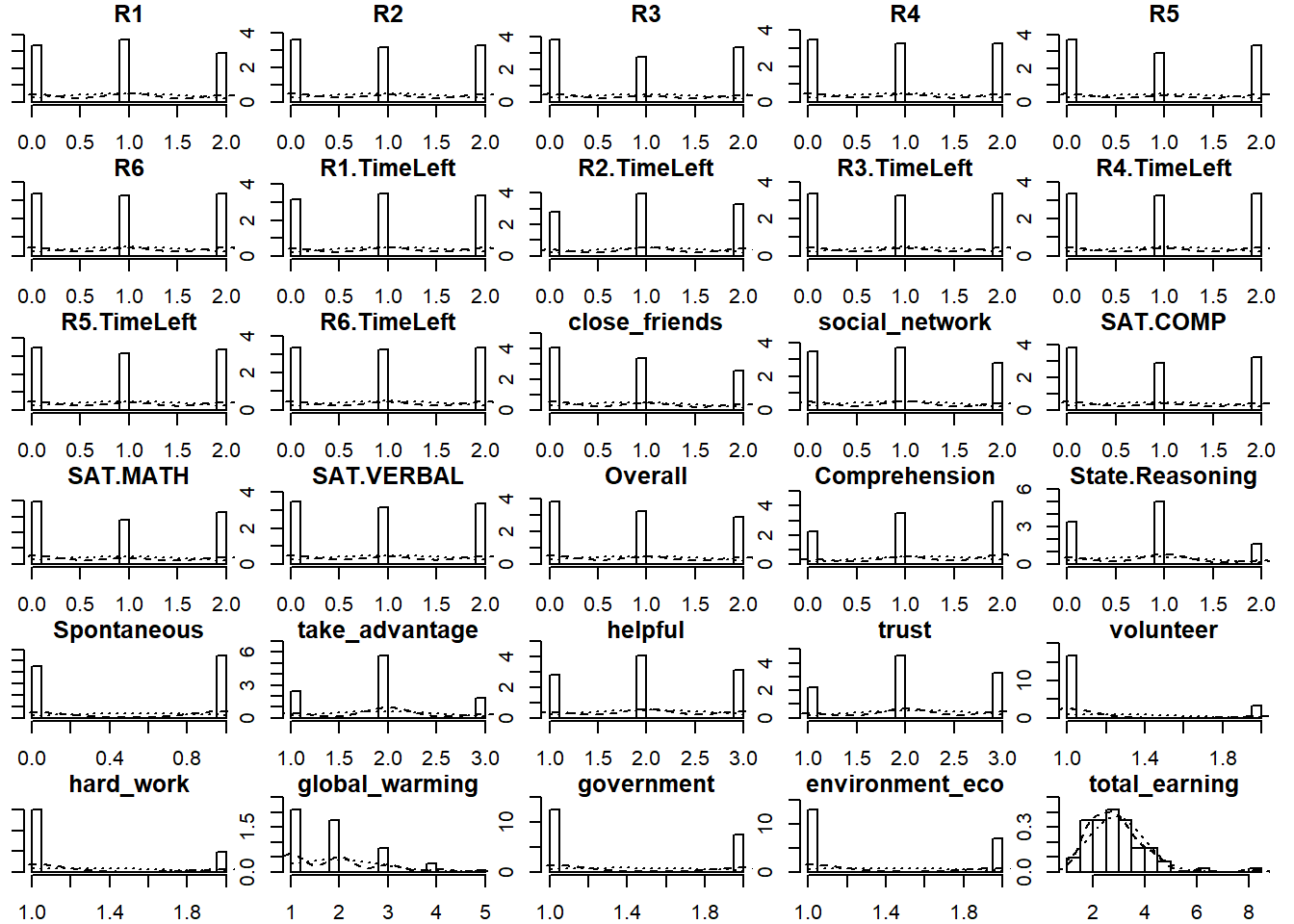
Figure 3.1: Histogram of Categorical Variables
3.2 Low Income Sausage
From this sausage data, we can know that there are five products and 27 emotional words. 20 Judges are required to evaluate these products by these words. The question is: How do you feel when you taste this product? Emotions were presented in a list, and consumers were able to choose as many emotions as they want.
# import data
low.income.sausage <- getURL("https://raw.githubusercontent.com/yilewang/MSA/main/Dataset/6Lowincomesausages.csv")
table.sausage <- read.csv(text = low.income.sausage)
colnames(table.sausage)[1] <- "Product"
kable(head(table.sausage[, 1:5]), align = "c")| Product | Happy | Pleasantly.surprised | Unpleasantly.surprised | Salivating |
|---|---|---|---|---|
| Alpino | 27 | 21 | 11 | 19 |
| Bafar | 28 | 20 | 6 | 19 |
| Chimex | 26 | 20 | 7 | 12 |
| Capistrano | 32 | 16 | 6 | 15 |
| Duby | 33 | 17 | 9 | 12 |
3.3 Wines
There are several wines from two places: South Africa and France. The wines table includes all the rating from Judges; The wines.name is table with list of emotional words in English and French; The wines.flavors table is some emotional words which are used to describe these wines.
# import data
wines <- getURL("https://raw.githubusercontent.com/yilewang/MSA/main/Dataset/Data_sorting_tri_fr_no_info_translate.csv")
wines.names <- getURL("https://raw.githubusercontent.com/yilewang/MSA/main/Dataset/Dictionary.csv")
wines.flavors <- getURL("https://raw.githubusercontent.com/yilewang/MSA/main/Dataset/Voc.csv")

table.wines <- read.csv(text = wines)
table.wines.names <- read.csv(text = wines.names)
table.wines.flavors <- read.csv(text = wines.flavors)

### Avoid UTF-8 error
colnames(table.wines)[1] <- "X"
colnames(table.wines.names)[1] <- "French"
colnames(table.wines.flavors)[1] <- "X"


kable(head(table.wines[, 1:5]), align = "c")| X | J1 | J2 | J3 | J4 |
|---|---|---|---|---|
| FCAR | 4 | 2 | 4 | 1 |
| SRUD | 3 | 4 | 3 | 1 |
| FBAU | 5 | 4 | 2 | 2 |
| FROC | 4 | 1 | 4 | 1 |
| SFED | 5 | 4 | 2 | 1 |
| SREY | 1 | 1 | 4 | 3 |
| French | English |
|---|---|
| acide | acidic |
| peu acide | low acidity |
| agressif | aggressive |
| agrumes | citrus |
| agréable | pleasant |
| alcool | alcohol |
| X | acide | peu.acide | agressif | agrumes |
|---|---|---|---|---|
| FCAR | 5 | 2 | 0 | 2 |
| SRUD | 4 | 3 | 0 | 2 |
| FBAU | 2 | 5 | 0 | 0 |
| FROC | 7 | 1 | 0 | 0 |
| SFED | 6 | 2 | 1 | 2 |
| SREY | 7 | 2 | 1 | 1 |